Showing posts with label Pandas. Show all posts
Wednesday, March 9, 2016

Tweets Analysis with Python and NLP


Introduction

You should be already familiar with the concepts of NLP from our previous post, so today we'll see more useful case of analysis the tweets and classifying them into marketing and non-marketing tweets. We won't get into details of tweets retrieval, this can be done with various packages with Tweepy being the most popular one.

Baseline

For the purpose of the discussion we already have 2 sets of tweets separated into files and are uploaded into GitHub folder. First we download the datasets, add target column as 1 for marketing tweets and unite the datasets. Then we'll check the baseline classification results, without any pre-processing. We do this so later we could understand whether our changes improve the metrics. We'll be using Random Forest for classification, since it doesn't expect linear features or even features that interact linearly and it can handle very well high dimensional spaces as well as large number of training examples. Plus it doesn't require a lot of configuration. Have a look at Random Forest and classifier boosting articles for more details.

# -*- coding: utf-8 -*-
import re
import numpy as np
import pandas as pd
from nltk.tokenize import WordPunctTokenizer
from sklearn.cross_validation import cross_val_predict
from sklearn.ensemble import RandomForestClassifier
from sklearn.feature_extraction.text import CountVectorizer
from sklearn.metrics import f1_score, accuracy_score, roc_auc_score

prefix = 'https://github.com/aie0/data/blob/master/tweets/'
badMarketingTweetsURL = prefix + 'bad_marketing_tweets.txt'
goodMarketingTweetsURL = prefix + 'good_non_marketing_tweets.txt'

vectorizer = CountVectorizer(max_features=5000)
tokenizer = WordPunctTokenizer()

# load ds
badMarketingTweetsDS = pd.read_csv(badMarketingTweetsURL, sep='\t',
                                   encoding='utf-8',
                                   names=['ID', 'Content'])
goodMarketingTweetsDS = pd.read_csv(goodMarketingTweetsURL, sep='\t',
                                    encoding='utf-8',
                                    names=['ID', 'Content'])

# marking target
badMarketingTweetsDS['isMarket'] = pd.Series(np.ones(len(badMarketingTweetsDS)),
                                             index=badMarketingTweetsDS.index)
goodMarketingTweetsDS['isMarket'] = pd.Series(np.zeros(len(goodMarketingTweetsDS)),
                                              index=goodMarketingTweetsDS.index)

X = badMarketingTweetsDS.append(goodMarketingTweetsDS)
y = X['isMarket']
X = X['Content']

def test_RF(transformator, options={}):
    tweets = transformator(X, options)
    features = vectorizer.fit_transform(tweets).toarray()

    y_pred = cross_val_predict(RandomForestClassifier(verbose=3,
                                                      n_estimators=100,
                                                      max_depth=10,
                                                      n_jobs=-1), features, y)
    acc = accuracy_score(y, y_pred)
    roc = roc_auc_score(y, y_pred)
    return acc, roc, f1


# 1. baseline
def transform_tweets1(tweets, options):
    return tweets

print(test_RF(transform_tweets1))
# (0.83827723901882489, 0.83818275302681977, 0.8342105263157894)
pass

Please notice the header of the file, # -*- coding: utf-8 -*-. Since tweets contain non-ascii characters, according to PEP 263, we should mark the file as such.

Our pipeline consists of 3 phases: pre-process the tweets (currently doing nothing), vectorizing the tweets and training the classifier using cross-validation to avoid overfitting. For details about cross-validation, read appropriate paragraph in linear regression article

We need vectorization since classifier cannot work with words and requires numeric vectors. To achieve the goal, we use scikit-learn CountVectorizer class, which implements bag of words technique.

Using no pre-processing we achieve 0.83 accuracy. Remember to check F1 and ROC metrics as well to spot skewed datasets, for more details see machine learning metrics article.

Pre-processing

Let's try several things to see what effect our changes have on the metrics.

def transform_tweets2(tweets, options):
    results = []
    length = len(tweets)
    i = 0
    for tweet in tweets:
        if i % 100 is 0:
            print("%d of %d\n" % (i, length))
        i += 1
        s = tweet.lower()

        if 'markEmoji' in options:
            try:
                s.decode('ascii')
            except:
                new_str = ''
                for l in s:
                    new_str += (" VGEMOJINAME " if ord(l) > 128 else l)
                s = new_str

        if 'patterns' in options:
            for (pattern, repl) in options['patterns']:
                s = re.sub(pattern, repl, s)

        words = tokenizer.tokenize(s)
        if 'remove_stop_words' in options:
            stops = set(stopwords.words("english"))
            result = " ".join([w for w in words if not w in stops])
        else:
            result = " ".join([w for w in words])
        results.append(result)
    return results

Removing stop words

We've all been taught that removing the stop words should the first step of any NLP pipeline. So that's only natural we start by doing so. The performance however not only hasn't improved, but actually showed a significant decline. Remember that we always should take into account the total number of instances when interpreting the performance, thus 0.834 - 0.822 = 0.012 decrease at 7000 instances is about 90 cases, which is a lot.

options = {
    'remove_stop_words': True
}
print(test_RF(transform_tweets2, options))
#(0.82943525385054195, 0.8290763420757612, 0.82242424242424241)

Marking links

Since removing the stop words didn't help, let's try something else - all links in tweeter are encoded, they don't provide any additional information and may only worsen the performance. Let's replace all links with hardcoded string VGLINKNAME. The performance increases by nearly 1 percent - good start!

replacement_patterns = [
    (r"http:\/\/t.co\/[a-zA-Z0-9]+", " VGLINKNAME ")
]
options = {
    'patterns': [(re.compile(regex), repl) for (regex, repl) in replacement_patterns]
}
print(test_RF(transform_tweets2, options))
#(0.84811751283513981, 0.84782082009277737, 0.85790527018012008)

Marking money

Marketing content usually contains monetary strings like "Win 100$". Let's try identify them and mark then with VGMONEYNAME. And the result - another percent up.

replacement_patterns = [
    (r"http:\/\/t.co\/[a-zA-Z0-9]+", " VGLINKNAME "), #link
    (r'\$\s{0,3}[0-9,]+', ' VGMONEYNAME ') # money
]
patterns = [(re.compile(regex), repl) for (regex, repl) in replacement_patterns]
options = {
    'patterns': [(re.compile(regex), repl) for (regex, repl) in replacement_patterns]
}
print(test_RF(transform_tweets2, options))
# (0.85667427267541363, 0.85637385309532066, 0.86601786428476202)

Marking Emojis

How about emotions? Do non-marketing emails contain more emotions through the use of Emojis signs? Let's try to create a feature around this idea by marking all non-ascii characters as VGEMOJINAME and check the results. Again the increase in performance by around half percent.

replacement_patterns = [
    (r"http:\/\/t.co\/[a-zA-Z0-9]+", " VGLINKNAME "), #link
    (r'\$\s{0,3}[0-9,]+', ' VGMONEYNAME ') #money
]
patterns = [(re.compile(regex), repl) for (regex, repl) in replacement_patterns]
options = {
    'patterns': [(re.compile(regex), repl) for (regex, repl) in replacement_patterns],
    'markEmoji': True
}
print(test_RF(transform_tweets2, patterns))
#(0.85853850541928122, 0.85730503637390198, 0.87023249526899159)

Conclusions

We can check more different ways to improve the performance, some will work, others won't. The main point you should take from this article is always rely on the data, never on what people say. Removing stop words may be a good idea in some domains and worsen the performance in others. Validate every assumption and play with the data as many as possible. Good luck!

Monday, February 8, 2016

Natural Language Processing with Python


Introduction

Natural language processing, or NLP, is a process of analyzing the text and extracting insights from it. It is used everywhere, from search engines such as Google or Bing, to voice interfaces such as Siri or Cortana. The pipeline usually involves tokenization, replacing and correcting words, part-of-speech tagging, named-entity recognition and classification. In this article we'll be describing tokenization, by using a full example from Kaggle notebook. The full code can be found on GitHub repository.


Installation

For the purposes of NLP, we'll be using NLTK Python library, a leading platform to work with human language data. It provides easy-to-use interfaces to over 50 corpora and lexical resources such as WordNet, along with a suite of text processing libraries for classification, tokenization, stemming, tagging, parsing, and semantic reasoning, wrappers for industrial-strength NLP libraries. Installing the package is easy using the Python package manager:

pip install nltk

Implementation

Let's walk through the Kaggle notebook and see that we understand what is done there. We'll be using already covered packages like Pandas, Scikit-Learn and Matplotlib. In addition we'll be using Seaborn, Python visualization library based on Matplotlib, which of course can be installed using the Python package manager:

pip install seaborn

The notebook analyzes the US baby names data between 1880 and 2014 and will be looking into questions how frequency occurrence of names in Bible correlate with US baby names. Firstly we'll load the data located in CSVs files, using Pandas read_csv method. To extract the names from the bible, the use of NLTK is done by taking advantage of nltk.tokenize package. Since we need all words staring with capital letter, we'll construct an appropriate regular expression rule. More about regular expression syntax can be found here.

nationalNamesDS = pd.read_csv(nationalNamesURL)
stateNamesDS = pd.read_csv(stateNamesURL)

bibleNamesDS = pd.read_csv(bibleNamesURL)
# retrieve all words starting with capital letter and having atleast length of 3
tokenizer = RegexpTokenizer("[A-Z][a-z]{2,}")
# load new testament
file = open(newTestamentURL)
bibleData = file.read()
file.close()
newTestamentWordsCount = pd.DataFrame(tokenizer.tokenize(bibleData))
.apply(pd.value_counts)

# load old testament
file = open(oldTestamentURL)
bibleData = file.read()
file.close()
oldTestamentWordsCount = pd.DataFrame(tokenizer.tokenize(bibleData))
.apply(pd.value_counts)

NLP is never used by itself and usually you'll want to some pre-processing prior to analyzing with text. Using Pandas drop and merge methods, we'll remove irrelevant columns and join the Bible capital words with known names from the Bible:

# remove irrelevant columns
stateNamesDS.drop(['Id', 'Gender'], axis=1, inplace=True)
nationalNamesDS.drop(['Id', 'Gender'], axis=1, inplace=True)

# retrieve unique names count of each testament
bibleNames = pd.Series(bibleNamesDS['Name'].unique())
# filtering out Bible names
newTestamentNamesCount = pd.merge(newTestamentWordsCount,
pd.DataFrame(bibleNames), right_on=0, left_index=True)
newTestamentNamesCount = newTestamentNamesCount.ix[:, 0:2]
newTestamentNamesCount.columns = ['Name', 'BibleCount']

oldTestamentNamesCount = pd.merge(oldTestamentWordsCount,
pd.DataFrame(bibleNames), right_on=0, left_index=True)
oldTestamentNamesCount = oldTestamentNamesCount.ix[:, 0:2]
oldTestamentNamesCount.columns = ['Name', 'BibleCount']

Great, now that we have our data, let's plot it with Matplotlib:

# plot top TOP_BIBLE_NAMES old testament names
topOldTestamentNamesCount = oldTestamentNamesCount.sort_values('BibleCount', ascending=False).head(TOP_BIBLE_NAMES)
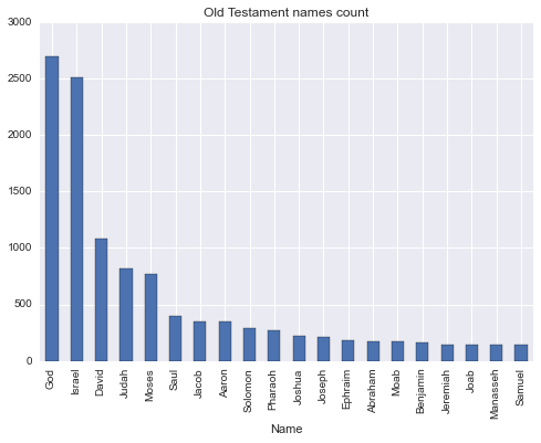
topOldTestamentNamesCount.plot(kind='bar', x='Name', legend=False, title='Old Testament names count')

DataScience is not just applying some already written algorithms and plotting the results. The insight to the domain is required to make a valuable and meaningful decisions. Otherwise we could just use Amazon Machine Learning. Using this knowledge, we understand that two the most frequent names are 'God' and 'Israel' should be removed. 'God' is not really a name, even though there is a statistically insignificant number of babies with this name in US. Despite 'Israel' being a name, it's also a country, of which Old Testament is all about.

oldTestamentNamesCount = oldTestamentNamesCount.drop(oldTestamentNamesCount[(oldTestamentNamesCount.Name == 'God') | (oldTestamentNamesCount.Name == 'Israel')].index)

After the pre-processing stage, the analysis starts. We wanted to see the correlate of frequency occurrence, so for this we'll be using Pearson correlation by Pandas corr method and plotting the data using Seaborn package. Why? The Matplotlib package, despite being a great one, doesn't provide very easy to use interface to plotting a scatter plot with colored categories. So, to ease our life, we'll use another package which supports exactly that. Have a close look at the code in lines 7-9. Since scatter plot method requires 2 dimensional data, we have to make our data such, by removing and flattening the data using Pandas unstack and reset_index methods.

# scale and calculate plot states with high corr
def plotStateCorr(stateNamesCount, title):
    stateNamesCount[['Count','BibleCount']] = stateNamesCount[['Count','BibleCount']].apply(lambda x: MinMaxScaler().fit_transform(x))
    stateNamesCount = stateNamesCount.groupby(['Year', 'State']).corr()
    stateNamesCount = stateNamesCount[::2]
    highCorrStateNamesCount = stateNamesCount[stateNamesCount.Count > HIGH_CORR_THRESHOLD]
    highCorrStateNamesCount.drop(['BibleCount'], axis=1, inplace=True)
    highCorrStateNamesCount = highCorrStateNamesCount.unstack()
    highCorrStateNamesCount = highCorrStateNamesCount.reset_index()
    fg = sns.FacetGrid(data=highCorrStateNamesCount, hue='State', size=5)
    fg.map(pyplot.scatter, 'Year', 'Count').add_legend().set_axis_labels('Year', 'Correlation coefficient')
    sns.plt.title(title)

plotStateCorr(newTestamentStateNamesCount, 'Correlation of New Testament and US state names')
plotStateCorr(oldTestamentStateNamesCount, 'Correlation of Old Testament and US state names')
oldTestamentStateNamesCount = None
newTestamentStateNamesCount = None
stateNamesDS = None

Similar stages of pre-processing is done on national scale, without any particular interesting difference, so we'll be ending our discussing at this point. You can of course follow the Kaggle notebook code and explanation till the end.

Conclusion

NLP with the assistance of NLTK library, provides us with tools, which open a huge spectrum of possibilities to us, previously only available to linguists professionals. In this article we've taken a glimpse at what NLTK does, by using tokenization tools. In the next articles we'll cover other aspects of NLP.

Monday, April 13, 2015

Python for Data Scientists - Pandas


Introduction

Having learnt NumPy and SciPy in previous articles, let's discuss our next package, called pandas.
Pandas provides rich data structures and functions designed to make working with structured data fast, easy, and expressive. It is, as you will see, one of the critical ingredients enabling Python to be a powerful and productive data analysis environment.

Pandas combines the high performance array-computing features of NumPy with the flexible data manipulation capabilities of spreadsheets and relational databases (such as SQL), mingling DataFrame - a two-dimensional tabular, column-oriented data structure with both row and column labels. It provides sophisticated indexing functionality to make it easy to reshape, slice and dice, perform aggregations, and select subsets of data.

For users of the R language for statistical computing, the DataFrame name will be familiar, as the object was named after the similar R data.frame object. However the functionality provided by R is merely a subset of that provided by the pandas DataFrame.

Installation

Installation of pandas is as everything in Python ecosystem, a piece of cake. For those working with Python distribution, it's been pre-packed for you. To install it manually using python package manager

pip install pandas

Data Structures

To get started with pandas, you will need to get comfortable with its two data structures used throughout the library: Series and DataFrame. I won't get into details about Panel and Panel4D, somewhat less-used containers, of which you can read on pandas site.

A Series is a one-dimensional array-like object containing an array of data (of any NumPy data type) and an associated array of data labels, called its index.

import pandas as pd
import numpy as np
pd.Series([1,3,5,np.nan,6,8])

# 0     1
# 1     3
# 2     5
# 3   NaN
# 4     6
# 5     8

A DataFrame represents a tabular, spreadsheet-like data structure containing an or- dered collection of columns, each of which can be a different value type (numeric, string, boolean, etc.).

dates = pd.date_range('20130101',periods=6)
pd.DataFrame(np.random.randn(6,4),index=dates,columns=list('ABCD'))
#                    A         B         C         D
# 2013-01-01  0.469112 -0.282863 -1.509059 -1.135632
# 2013-01-02  1.212112 -0.173215  0.119209 -1.044236
# 2013-01-03 -0.861849 -2.104569 -0.494929  1.071804
# 2013-01-04  0.721555 -0.706771 -1.039575  0.271860
# 2013-01-05 -0.424972  0.567020  0.276232 -1.087401
# 2013-01-06 -0.673690  0.113648 -1.478427  0.524988

As you can see DataFrame has both a row and column index; it can be thought of as a dict of Series.

Examples

Index Objects

As we've seen in the DataFrame example, we can provide a custom index to both DataFrame and Series objects and then reference items through by using it.
s = Series(range(3), index=['a', 'b', 'c'])
s['a'] # 0
s['b'] = 16.5

Reindexing

Consider a case, where you'd like to change the indices of your data resulting alternation, addition or removal of entities.
index = ['a', 'c', 'd']
columns = ['GBP', 'USD', 'EUR']
data = np.arange(9).reshape((3, 3))      # reshape 9x1 to 3x3
frame = DataFrame(data, index=index, columns=columns)
#   GBP USD EUR
# a 0   1   2 
# c 3   4   5
# d 6   7   8

frame.reindex(columns=['GBP', 'JPY', 'EUR'])
#   GBP JPY EUR
# a 0   NaN   2 
# c 3   NaN   5
# d 6   NaN   8

frame.drop('GBP')
#   JPY EUR
# a NaN   2 
# c NaN   5
# d NaN   8

As you can see, both adding and removing indices is as easy as breathing. Both methods support array parameters, so bulk data alternation is also possible and even advisable from optimization purposes.

Arithmetic and data alignment

Another important pandas feature is arithmetic behavior between objects with different indexes. When adding together objects, if any index pairs are not the same, the respective index in the result will be the union of the index pairs.

s1 = Series([7.3, -2.5, 3.4, 1.5], index=['a', 'c', 'd', 'e'])
s2 = Series([-2.1, 3.6, -1.5, 4, 3.1], index=['a', 'c', 'e', 'f', 'g'])
s1 + s2
# a 5.2
# c 1.1
# d NaN
# e 0.0
# f NaN
# g NaN

Here column d, f and g were converted to NaN as they didn't have a match in both series. The same applies to DataFrames of course. One thing you might find useful is filling the NaN values with some defaults. This can be achieved using filling function, supported by all corresponding methods: add, sub, div and mul.

Merge

What about morphing 2 data objects. No worries - pandas comes to rescue. It provides various facilities for easily combining together objects with various kinds of set logic for the indexes and relational algebra functionality in the case of join / merge-type operations.

key = ['foo', 'foo']
left = pd.DataFrame({'key': key, 'lval': [1, 2]})
#    key  lval
# 0  foo     1
# 1  foo     2

right = pd.DataFrame({'key': key, 'rval': [4, 5]})
#    key  rval
# 0  foo     4
# 1  foo     5

pd.concat([left,right])
#    key  lval  rval
# 0  foo     1   NaN
# 1  foo     2   NaN
# 0  foo   NaN     4
# 1  foo   NaN     5

merged = pd.merge(left, right, on='key')
#    key  lval  rval
# 0  foo     1     4
# 1  foo     1     5
# 2  foo     2     4
# 3  foo     2     5

merged.groupby('key').sum()
#      lval  rval
# key            
# foo     6    18

Handling Missing Data

Very often, if not always, we deal with incomplete data, either by it's nature like sensor data or as a result of human error like spreadsheets. Pandas provides various functionality to deal with such situations.

from numpy import nan as NA
data = Series([1, NA, 3.5, NA, 7])
data.dropna() # similar to data[data.notnull()]
# 0 1.0
# 2 3.5
# 4 7.0

data.fillna(0)
# 0 1.0
# 1 0.0
# 2 3.5
# 3 0.0
# 4 7.0

With every evolving API, pandas provides numerous functionality, which will ease any data scientist life. Make sure you keep yourself updated with the features of every release.